Short Selling at the height of Pandemic?

By Frederico Werner de Mascarenhas and Daniel Christian Henrique

The stock market in Brazil is still poorly accessed, according to the latest data from B3 (2019), there were 1,046,244 individuals registered until the end of April 2019. As an aggravation of this scenario, in the approached methodology, the investor is counted more than once, if he has more than one active account with a broker. For a country with a population of 209.9 million (IBGE, 2019), this number is very low compared to others, especially the more developed ones. According to Magliano Filho, (2002, p.1, our translation) “in Brazil we have a very small number of people participating in the stock market, while in the USA, 50% of families invest in the stock market; in England, this percentage reaches 30% ”.

Within the investor profile, according to a study by Santos Júnior (2012), individual investors tend to have few assets. Statman (2004) complements when stating that the average of US investors' assets is 3 to 4. Initial studies on the best risk x return ratio in traditional investment portfolios (without short selling) were developed by Evans and Archer ( 1968) and Statman (1987), followed later by Gupta, Khoon and Shahnon (2001), Elton, Gruber, Brown and Goetzmann (2012) and Chong and Phillips (2013). The conclusions indicate compositions that bear portfolios among 10 assets in the oldest researches with 31 shares in the most recent ones, which consequently already outlined a greater number of shares, sectors and complexity of investments in the stock exchanges.

There are, in addition, several methods for the composition of riskier or safer portfolios, not covered in these studies. Among the compositions that seek strategies with more aggressive returns and risks short selling stands out, in which the investor bets against the market. The studies by Chen, Chung, Ho & Hsu (2010), Michaud (1993), Grinold and Kahn (2000) and Kumar, Mitra and Roman (2008) indicate in the results that short selling portfolios permeate higher returns accordingly to the increase in risk percentages, without however indicating an optimal number of assets for this methodology. This study intends to advance from this point, offering an optimal frontier for short selling assets of a stock exchange in a developing market, in an attempt to gain in an efficient frontier that does not excessively extrapolate the risks to be assumed and become more an alternative in these periods of low fixed income earnings.

Taken, on the other hand, the inexpressive list of publications in this aspect of portfolios immersed in the national stock market, it is pertinent to question for this context applied to B3: (1) what is the maximum percentage of return x risk that it would be possible to obtain with an adequate work of diversification for the Long and Short strategy applied in the financial statements from 2015 to 2018 before the covid-19 pandemic and projected for a future period of 3 years (until 2021)? Then, compare it with a new projection of these data during the peak of the pandemic, with a projection for until 2023. Would it still be possible to obtain returns with higher risk investments in this diversification adopted in such a critical period?

A medium-term period was chosen in view of the only recent increase in popularization of variable income investment in the pre-pandemic period, which is still a novelty for many, leading to shorter terms for their exit from the market. On the other hand, strong diversification is necessary in view of the still low number of people registered on the stock exchange and the concentration of their trades in a few assets, aiming to gradually reduce the increase in risks by applying it to different amounts of assets in the portfolio. With even more pronounced declines in fixed income, as well as variable income, during the pandemic, this need became even more necessary.

The other emerging questions are: (2) what, then, is the ideal number of shares for diversification of Long and Short portfolios applied to B3? (3) is this number forming a more complex or simpler portfolio than those that make up portfolios without short selling? (4) what is the difference in the loss of profitability for this optimum number before and during the pandemic? Based on the premise that the rational investor is risk averse and tends to maximize his returns with the lowest risk levels (REILLY, NORTON, 2008) and that consequently those who seek a higher return will tend to bear greater risks, this study will search for assets that satisfy these conditions and answer these questions.

In order to achieve these objectives, metrics of fundamental analysis were approached, which stipulates the analysis of the true value of the shares (PINHEIRO, 2009) and subsequent choice of the best assets from healthy companies that generate returns over the long term - as long as their fundamentals are maintained over time - for the composition of portfolios. This type of analysis permeates an adequate diversification and reduces the non-systematic risk of a portfolio, since a specific asset can be counterbalanced by the specific variability of the other assets (REILLY, NORTON, 2008). The efficient frontiers of the portfolios were developed using the Economatica software, which adopts the Markowitz model for projections, adapted to the possibility of short selling (ECONOMATICA, 2019) in line with the use of asset restrictions.

Markwotiz model for Portfolio Optimization

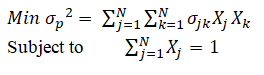
Chen et al. (2010) describe that the Markowitz portfolio model (called the average variance) is one in which no further diversification can reduce the portfolio's risk to a certain expected return. Alternatively, no expected excess returns can be obtained without increasing the portfolio's risk. This conception is based on a series of hypotheses, listed below (MARKOWITZ, 1952): 1) the distribution of the probability of expected returns in a period, is possible to be determined; 2) investors have single-period utility functions, in which they maximize it; 3) the variability on possible expected return values is used by investors to measure risk; 4) investors are only concerned with the averages and the variation in the returns of their portfolios during a specific period; 5) the expected return and risk used by investors, are measured by the first two deviations from the probabilistic distribution of the expected return and variance; 6) the return is desirable; the risk must be avoided; 7) financial markets are frictionless.

From the model result, the concept of efficient frontiers emerges: a set of all portfolios in which the expected returns reach their maximum value, for a given level of risk. This punctuated, it is incurred that the Markowitz optimization problem can be solved for different objectives and restrictions, as desired by the investor, and can be written according to the following model (CHEN ET AL., 2010):

For Michaud and Michaud (2008), the traditional Markowitz model features some limitations and should be adjusted according to the preference restrictions of investors. They postulate that the input data must be well worked to generate a good optimization job, as, for example, via the selection of assets based on their fundamentals. Another way normally used by investors, listed by the authors, is the addition of linear inequalities to restrict asset weights. In this way, the optimization of the portfolio avoids the concentration in certain assets, or economic sectors, as the concentration tends to harm the diversification work. A model without proper adjustments can be ineffective, damaging the investor. Reilly and Norton (2008) also remind investors that they can benefit from the sector rotation strategy when only domestic assets are obtained, taking the benefits of market movements by increasing or decreasing the weights of assets according to the phases of the economic cycle.

An adaptation of the analytical representation of the weight restriction of the assets of Rubesam and Beltrame (2013) can be written according to the inequality (2). Therefore, it should be inserted in the objective function of the traditional Markowitz model (1), as one of the restrictions of the problem.

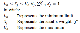
According to Fan, Zhang and Yu (2012), the development of equity funds always involves individual asset restrictions. This is commonly understood as an effort to reduce portfolio risk.

Short Sale

In the stock market when an investor buys an asset in the hope of its appreciation, it is recurrent to say that the investor is buying (long). On the other hand, investors can sell assets they do not own, renting it from the market, to later buy at lower prices and gain from the falling market. This practice is called short sale (ELTON ET AL., 2012). When the investor practices short selling, it is labeled that it is sold (short). Therefore, the investor who lent the shares has the proceeds of the sale as collateral, just as he can invest the funds obtained in risk-free securities (REILLY, NORTON, 2008).

The investment fund industry commonly uses the short sele strategy. According to ANBIMA (2015), a fund that uses bought and sold positions can be classified as Long and Short; the Long Biased terminology applies when maintaining at least 67% of the purchased portfolio. The fund that practices only bought positions is called Long Only.

The traditional Markowitz model does not use the Long and Short strategy, that is, it does not allow negative weights for the assets. At the time of writing, this possibility of composing portfolios was far from investors. However, with the advancement of computational tools and reduced transaction costs, this strategy has become economically viable, gaining popularity among investors (Michaud & Michaud, 2008).

Michaud (1993) states that the Long and Short strategy is capable of providing greater returns to the investor, but accompanied by greater risks. Its benefit comes from the removal of the negative weight restriction on assets, offering investors the possibility of leverage (Michaud, 1993; Grinold & Kahn, 2000). Such a strategy is aimed at a specific niche of investors who accept greater risks in the possibility of greater returns, since at the point of sale the loss limit tends to infinity, in addition to expanding possibilities of choice in the decisions of your portfolio (MICHAUD, 1993; KUMAR, MITRA, ROMAN, 2008).

Grube and Beedles (1968) contribute to a comparative study between a simplified Long Only portfolio (including short sale restrictions) with another portfolio without restrictions. Among the results, they found that an unrestricted short selling portfolio has higher returns per risk unit compared to a restricted one.

On the same theme, Grinold and Kahn (2000) conclude that there is an increase in the effectiveness of the Long and Short strategy in relation to the Long Only strategy, taking as a definition of effectiveness the expected excess return coefficient of the portfolio (α), in relation to Long Only strategy. They add that such a Long and Short strategy is effective when the universe of assets is large, the volatility of assets is low and the investment strategy has a high degree of active risk. In a more recent study, Kumar, Mitra and Roman (2008) collaborate by stating that this format of portfolio composition provides better risk and return relationships, for certain proportions, in relation to the Long Only strategy.

Analytically, the Markowitz model with the implementation of short sale, can be written according to the operational research problem (Francis, 2010):

Using the constraint, allows the model to assign negative weights to assets (short sale), but maintains the requirement that the absolute total amount of money invested be equal to 1. The solution to the problem is similar to the traditional model and the Lagrange C function, according to equation (4) (Francis, 2010):

In a similar way, the solution of the problem is driven by taking the partial derivatives of the function C in relation to each weight variable (Xj), of each Lagrange multiplier (λ), to finally offer its result equal to zero. Francis (2010) writes the result of the equations in the form of a matrix, as shown:

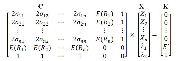
   To solve the matrix:

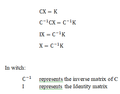
The solution will provide the respective weights for each asset as a function of the expected return E´. As a result, for different returns, the efficient frontier for short selling can be drawn. Kirch (2018) additionally corroborates when proposing the use of the penalty function algorithm, in addition to linear programming, for the problem of solving short selling restrictions.

One of the most used ways for this strategy is through the imposition of a total limit of 30% of the portfolio with short sales, called strategy 130/30. Lo and Patel (2008) state that in the investment fund industry in the United States, the 130/30 strategy is among the fastest growing in the applications of managers. In Brazil, ANBIMA (2015) classifies these funds as Long Biased. In its operation, the manager is leveraged in a proportion of 1.6, when short selling 30% of the portfolio and being bought in 130% with the money obtained from the market. For example: starting from a portfolio with $ 100,000, the manager can obtain $ 30,000 from the short sale and uses this money on the long end.

One of the reasons for limiting the total leverage of the portfolio comes from the United States stock market, which incurs a series of limitations imposed by the SEC (U.S. Securities and Exchange Commission) on investment funds (SEC, 2015). In Brazil's reality multimarket funds can be highly leveraged, with maximum leverage limits depending on the regulation of each fund (CVM, 2014).

Methodology

Methodological Steps

The research steps are listed below:

• Identification of the filters and rules that would be used in the composition of the best actions in each economic sector of B3. For the purposes of this research, the selection of assets was made through the Value Investing strategy using fundamentalist indicators, as seen below:

Table 1. Fundamentalist indicators chosen

• Data collection: using the previously established indicators, the Screening module of the Economática® software was used to collect all the data necessary for the treatments.
• Data treatment: 10 Excel® spreadsheets were created, each representing a B3 economic sector. With this stage completed, the shares were ranked as will be described in detail in section 3.2.
• Preparation of four portfolios, explained in section 3.3.
• Portfolio optimization: using the Economática® optimization module. Initially we entered values for weight restrictions of assets without verification.
• Asset weight restrictions test: the minimum and maximum asset weight restriction limits for each portfolio were empirically tested until reaching the restrictions that could achieve the highest returns, regardless of the risk level (however limiting the concentration of a certain asset). Portfolios with leverage restrictions were also tested: the 130/30 strategy.

Analysis and discussion of the results: With the results of the Economática® optimization module, it was possible to elaborate efficient borders with the help of Excel® to achieve the research objectives.

Identification of Filters for Portfolio Assembly

The identification of the filters for the assembly of the portfolios occurred in two stages: 1) application of initial filters in order to exclude companies that do not satisfy the pre-established conditions for the analyzes; 2) choice of indicators used for data treatment. Thus, some initial rules were established for the exclusion of companies with negative financial results: a) exclusion of companies with less than three years on the stock exchange; b) exclusion of companies with negative return on equity (ROE) in the last 12 months; c) elimination of the shares of companies with negative P / L and P / VPA indicators; d) companies with more than one trading code: the one with the most liquidity was chosen; e) exclusion of companies under judicial recovery or that are going public on the date of data collection; f) elimination of the shares of companies without data.

Further adjustments were still needed. For the “financial sector and others”, the indicators: Net Debt / EBITDA, EBITDA Margin, ROIC, PSR and EV / EBITDA, were excluded from the analysis due to the peculiarities of the sector. And finally, due to the fact that some of these indicators use the market price on the collection date, an average of the last 4 annual balance sheets (2018, 2017, 2016, 2015) was configured for all indicators, in order not to generate some bias in research. Table 2 shows the number of companies by economic sector that passed the filters.

Table 2. Number of Companies that passed the initial filters

The ranking system was made following the preference of direction of each indicator by profile. For example: for the company that had the highest Current Liquidity value, it received the number 1, as it is the one that best presents the ability to honor its obligations in the short term within its economic sector. The one with the second best value, got the number 2, and so on. Regarding the indicators that showed the opposite direction of preference, the logic remains: the lowest value receives the number 1 and so on. With all the scores established, the companies with the best ratings on the indicators were ranked in ascending order. In the event of a tie, the tiebreaker criterion was that which obtained the best ratings for the market indicators.

Portfolio Composition

With the ranking finished, the portfolio assembly process followed the following logic. Four portfolios were created with different amounts of assets: the number 1 portfolio was composed of the best shares in each sector, totaling 10 shares; portfolio 2 was assembled by the two best shares in each sector, totaling 20 shares; portfolio 3 with 30 shares; and, finally, portfolio 4 with 40 shares, following the same logic of assembly. The assets of each portfolio are those available in the table below:

Table 3. Portfolio Composition

Due to the fact that B3 does not have a large number of companies, the Telecommunications and Information Technology sectors did not have enough candidates. Thus, for filling portfolios 3 and 4, the logic was: to use companies from other sectors with a greater number of representatives, until the portfolios were completely filled.

Portfolio Optimization and Verification of Restrictions

Pre-pandemic: the input parameters for inserting the assets for the composition of the borders were those listed in sequence: projected return calculation method: CAPM; projected period: 3 years (2019 to 2021); risk-free asset: Selic Treasury (LFT); benchmark: Ibovespa; correlation calculation period: 36 months; restrictions: asset weight restriction module, allowing negative weights. Peak of the pandemic: ditto the previous one, but projected for from May 2020 until 2023.

Initially, weights restrictions of assets were inserted without verification, as it was not possible to know the result of efficient frontiers beforehand. Restrictions that could achieve the highest possible returns were tested, regardless of the level of risk, but without allowing excessive concentration on an asset. Restrictions are understood as the introduction of a minimum or maximum percentage for each asset in the composition of a portfolio, varying its weight from 0 to 100% without short selling. However, for portfolios short sold in a specific stock or set of shares, a minimum limit with a negative value equivalent to the percentage allowed for short selling must be introduced (ECONOMÁTICA, 2019).

It took 5 rounds until the objective was reached. The restrictions for each portfolio are shown in table 4.

Table 4. Restriction of Assets weights

For the 130/30 strategy, which limits the total leverage of the portfolio to 30% for short selling, the individual restrictions per asset were the same.

Results and discussions

Frontiers without Leverage Limits on Short Sale - Pre-pandemic

For borders without leverage limits, equipped with restrictions, it is obtained only by the minimum limit of individual assets. Figure 1 shows that for lower risk levels, portfolios with 3 and 4 assets go practically together; however, for higher levels of returns, portfolio 3 with 30 assets is slightly more efficient. This is due to the flexibility of asset restrictions, which offers the possibility for the investor to obtain higher returns through short selling and the possibility of concentrating on certain assets without being obliged to own all shares.

Figure 1. Efficient Short Selling Boundaries Projected by 2021 - No Leverage Limits

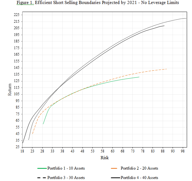
At higher risk levels, such as no 88% risk point, or an investor who joins portfolio 3 in exchange for portfolio 2, obtain a return of approximately 50% higher (with the same risk). A portfolio 3, therefore, that makes up the ideal number of assets (30 shares from a total of 104 eligible) within a context of diversification at B3, which responds better to the return records requested in the Long and Short composition. This average assessment is made by Grinold and Kahn (2000) on the need for a large volume of assets for the effectiveness of portfolios with undiscovered sales.

It is noteworthy that there was an increase in 10 assets between portfolio 1 and 2 occasionally, with a decrease of 18.58% without risk at the point of minimum variation. With regard to portfolio 3, the risk is reduced by 8.53% in relation 2; while the movement for portfolio 4, a reduction of 13.88%. Thus, the latter portfolio shows the best choice for an investor looking for lesser risks.

Another point highlighted for the variation in the weight of assets in figure 2, using portfolio 3 as an example. At the border points, where the risk and return ratio is lower, a significant part of the 30 assets that are being the upper part of the graph indicated that assets are included. With increasing returns, assets start to diverge. There is no return point of return of 185.70%, some assets of the portfolio use minimal limitation, register less than -20% of the portfolio and are represented by them.

Figure 2. Efficient Frontiers - Variation in the individual weights of the assets in Portfolio 3

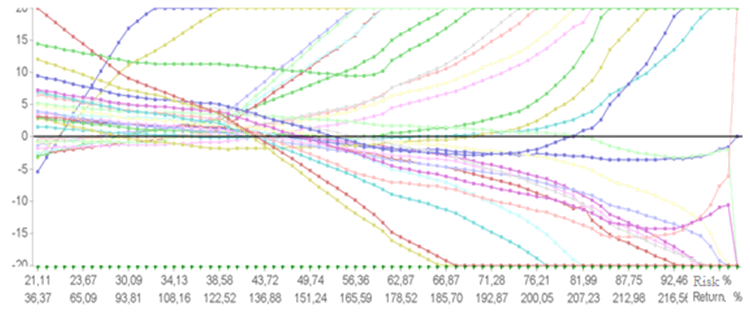
This variation confirms this topic in the Long and Short portfolio works by Michaud (1993), Grinold and Kahn (2000) and Kumar, Mitra and Roman (2008), showing that greater returns are possible due to the elimination of restrictions on short selling.

Short Selling X No Short Selling - Pre-pandemic

To test the effectiveness of short selling, the most efficient frontier portfolio, portfolio 3, was used to simulate three different restrictions in sequence. The first composed the locking of the minimum limit at 0%, that is, not allowing the portfolio to be sold, but maintaining the maximum limit at 15%. The second restriction addressed the 130/30 strategy, allowing the portfolio to be sold, but limited to 30% of the total. Finally, in the third restriction, the portfolios are left with no total leverage limit, as only individual asset restrictions are imputed. Table 5 summarizes the restrictions and figure 4 the result of efficient borders.

Table 5. Restrictions

Figure 3. Projected x short selling boundaries by 2021

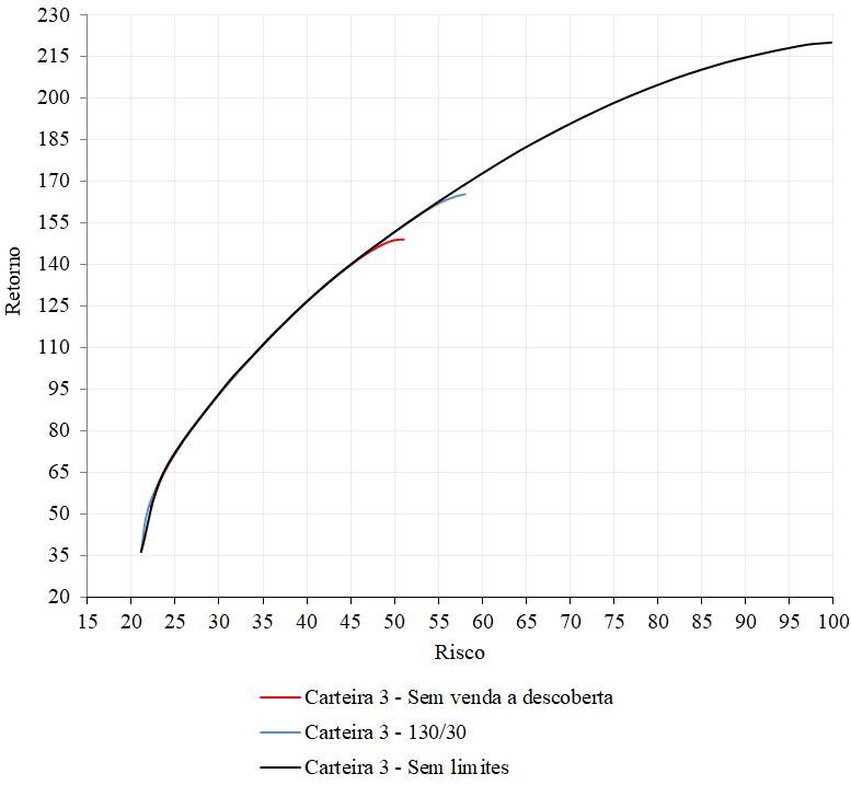
Becomes evident the similarity with the efficient borders obtained in the results by Chen et al. (2010) when short selling was introduced in the portfolio, as the extension of borders occurs as leverage increases. As shown in figure 4, the portfolio without short selling reaches the maximum return in the range of 149%, while the 130/30 strategy reaches a little more, around 165% and; finally, the portfolio without limits reaches values close to 220%. And yes, the increase in returns is accompanied by greater risks. This assumption, on the other hand, highlights the greater efficiency in certain points of risk of short selling. Using the 50% risk point as an example, it is noted that the portfolio with the easing of restrictions on short selling is more efficient.

In studies by Kumar, Mitra and Roman (2008) applied to the London Stock Exchange Index (FST100), they see a 17.82% gain between their Long and Short portfolio with a similar strategy (120/20) and the Long Only portfolio. Although the 130/30 strategy is slightly different, this modality of B3's diversified portfolio obtained a percentage of 16% in its comparative gain with Long Only, slightly lower than the previous study.

In order to verify the effectiveness of obtaining greater returns, some indicators were raised in order to compare the strategies and confirm the effectiveness of the short selling strategy. One of these is Jensen's Alpha, mentioned by Grinold and Kahn (2000). Table 6 shows the results:

Table 6. Statistical indicators at the point of maximum return

With the easing of restrictions, it is noted that the more leveraged the portfolio, the greater the chances of obtaining higher than expected returns. Jensen's Alpha projected for the Long and Short portfolio period is 7.94%, approximately five times higher than the Long Only strategy. Consequently, the risk of the Long and Short strategy portfolio is greater, since the probability of loss in 1 day at a 95% confidence level (VaR) is 5.96%, while for the Long Only strategy it is 3.05%. It is also noteworthy that the observed beta of the Long and Short strategy is greater than the betas of the other two strategies, indicating that the first moves 1.388 times the movement of the Ibovespa Benchmark. As for the correlation, the Long and Short portfolio is the one with the lowest value, indicating that the strategy is interesting for an investor who seeks to de-correlate from the market index. Thus, an investor can obtain good returns with the short selling strategy.

Frontiers Without Leverage Limits on Short Sale – Height of pandemic

After confirming the effectiveness of the portfolio with 30 assets in the pre-pandemic period (before 2019), the same four portfolios were created with the same number of shares, but launched in early June 2020 with projection for the next three years taking as the same companies selected in the previous period. The maintenance of these assets is justified by their choice, based on the performance of their financial indicators. Until December 2018, the fundamentals of companies were not guided by drastic fluctuations in political moments of election or the pandemic. This allows us to consider that these are still the most financially grounded corporations for investment choices during the height of the pandemic, even with their shares below their expected prices. It would be impossible to make a concrete investigation of financially sound companies in a situation of high volatility at the height of the pandemic, when the news of a daily increase in contamination still impacted the Ibovespa index frequently (although it has already slowly and gradually resumed some growth against the bottom reached in March 23, but still very unstable), with Brazil in second place in the world ranking of contaminated, reaching a total of more than one million contaminated on June 20, with continuous exponential daily growth of cases. Some assets were reclassified in B3 in this period:

• Former: Kroton (KROT3). New: Cogna (COGN3)
• Former: Queiroz Galvao (QGEP3). New: Enauta (ENAT3)
• Former: Sierrabrasil (SSBR3). New: Aliansce Sonae Shopping Centers (ALSO3)

              In sequence as portfolios optimized with new projections without leverage limits:

Figure 4 Efficient Short Selling Boundaries Projected by 2023 - Peak of the pandemicprojetadas até 2023 - Auge da pandemia

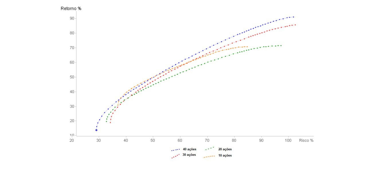
Initially, one can already see a drastic drop in the profitability of the four portfolios with an increase in the associated risks, reaching a maximum return of 90% (for a risk of 105%) obtained by portfolio 4 (with 40 shares), against 217% of portfolio 3 (100% risk) in the pre-pandemic period, denoting an exchange of portfolios in the maximum risk x return ratio. In summary, at the point of greatest risk-return ratio, exactly 127% of the previous yield was lost and the risk rate was increased by 5%, adding to the need to increase 10 stocks in the pre-pandemic portfolio to enable the greatest possible income at the height of the pandemic, showing greater need for diversification. Below is a comparative table between some points of both efficient borders:

Table 7. Comparison of Risk vs. Return of Portfolio 3 Pre-Pandemic and Portfolio 4 Height of Pandemic

Therefore, it is noted that the total sector diversification continued to be even more opportune, implying a not so significant drop in profitability at a time of severe economic crisis and the flight of investments from variable income to fixed income (mainly for savings) ) that the peak of the pandemic has established. The diversification with the total number of 40 assets made it possible to maintain almost the same level of risk, close to 100%, at the point of greatest return on the efficient frontier.

With the sharp drop also in the Selic rate and the consequent extremely low yields from the CDI, from savings applications, CDBs and direct treasury, the drastic expansion in this type of investment proved to be more opportune for many investors when associating the guarantees linked to the FGC (Credit Guarantor Fund) and flight from declines in variable income than effectively to some more profitable income. Emergency aid payments to millions of Brazilians also contributed to the jolt of savings entries, as many deposits were held back by bureaucratic and registration issues that made it impossible for many to withdraw their funds immediately, being automatically applied to savings.

On the other hand, it can be seen in the comparative results between pre and peak of the pandemic that investors more mature in diversification still had a good opportunity to maintain more attractive returns in the pandemic in their own variable income, even losing 2/3 of the total return in comparison previous period and needing to increase the number of assets.

It should also be noted that the rock bottom in the stock market is a key moment to make investments in variable income assets, in contrast to what herd investors do when migrating to fixed income. Ibovespa was in January / February in a happy time of great increases in the number of registered individual investors, fleeing the terrible performance that fixed income had been obtaining. However, with the news of the significant expansion of covid-19 in Brazil, many soon abandoned their new investment option with greater risks on the stock exchange. After the biggest drop, since March 23, the Ibovespa is showing a slow and gradual recovery, as can be seen in the graph below, being a great opportunity to leverage gains in the most financially based companies, which are more likely to follow the new upward trend of index scores:

Figure 5 - ARIMA (3, 1, 2) - Ibovespa projection for 60 days

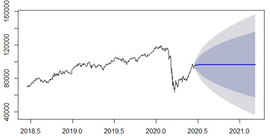
Therefore, measurements of daily projections are taken with a model formatted with daily data since the beginning of the year, denoted by the midline and dark and light gray areas with confidence levels, respectively, of 80% and 95%, little can be said about predictions in view of the sharp drop in February, the ARIMA model (3, 1, 2) being the best accepted in comparisons for AIC and BIC performance measures. The 3rd order projection with a differentiation and two moving averages to explain past errors was not enough to demonstrate a clearer path to follow. A projection with a horizontal line without trend was maintained, with the expected fluctuations in accordance with future pessimistic or optimistic scenes falling to the confidence levels. That said, an analysis focusing on the very short term of the recovery period, with an upward trend, started on March 23, for a more accurate prediction:

Figure 7 - ARIMA (0, 1, 0) and Holt forecasts for high period

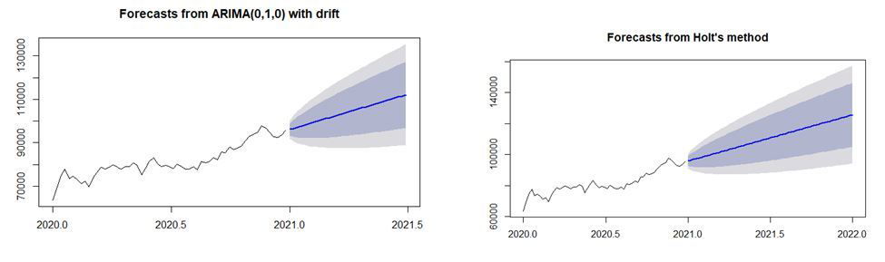
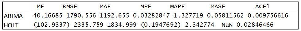
The absence of more specific patterns led to a similarity between the exponential adjustment projections (Holt) and that of an ARIMA (0, 1, 0), considering only a differentiation for the projections as the most accurate technique according to the results of their AIC and BIC. Taking as a parameter the comparison between the accuracy measures, the most appropriate model is ARIMA, presenting the lowest error values with its forecast.

Table 2 - Accuracy Measures for ARIMA (0, 1, 0) and Holt Models

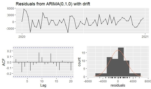
Observing the residues of the chosen model, its full validity for the predictions is confirmed. The Ljung-box test was approved, denoting residues in white noise, with a p-value equal to 0.7789, confirmed by the graphs of the time series of the residues together with the ACF, within the limits of significance, refuting any possible autocorrelation between the mistakes. In addition, normality was accepted by the Shapiro-Wilk test with a p-value equivalent to 0.8362, confirmed by the histogram graph.

Figure 8 - Residue analysis

Therefore, for those who are still looking for a more attractive return on high-risk variable income and an escape from almost zero profitability from current fixed income investments, full diversification between sectors in portfolios with assets exclusively allocated to short selling remains opportune, as confirmed the comparison of the pre and peak pandemic portfolios. The crisis reduced 2/3 of its profitability, but the diversification allowed it not to be even more, becoming a more robust return to more aggressive investor profiles, enhanced by the gradual upturn in the Brazilian stock market.

References

ANBIMA. Nova Classificação de Fundos -Visão Geral e Nova Estrutura, 1–19, 2015. Available in: https://www.anbima.com.br/data/files/E3/62/8C/0B/242085106351AF7569A80AC2/NovaClassificacaodeFundos_PaperTecnico_1_.pdf

ASSAF  NETO, A. Mercado Financeiro (12th ed.). São Paulo (SP): Atlas, 2014.

B3.BM&FBOVESPA Histórico pessoas físicas, 2019. Available in: http://www.b3.com.br/pt_br/market-data-e-indices/servicos-de-dados/market-data/consultas/mercado-a-vista/historico-pessoas-fisicas/

CHEN, W., CHUNG, H., HO, K., HSU, T. Portfolio Optmization Models and Mean-Variance Spanning Tests. In: LEE, C.-F.; LEE, A. C.; LEE, J. C. (Eds.).  Handbook of Quantitative Finance and Risk Management. 1 ed.  Springer, 2010. p. 165–184. https://doi.org/10.1007/978-0-387-77117-5

CHONG, J.; PHILLIPS, G. M. Portfolio Size Revisited. The Journal of Wealth Management, v. 15, n. 4, p. 49–60, 2013. https://doi.org/10.3905/jwm.2013.15.4.049

COMISSÃO DE VALORES IMOBILIÁRIOS. CVM No 555. n. 21, p. 120, 2014. Available in: http://www.cvm.gov.br/legislacao/instrucoes/inst555.html

DEMIRAKOS, E. G.; STRONG, N. C.; WALKER, M. What valuation models do analysts use? Accounting Horizons, v. 18, n. 4, p. 221–240, 2004. Available in : http://economatica.com/support/manual/portugues/whnjs.htm.

ECONOMATICA. Manual, 2019. Available in: http://economatica.com/support/manual/portugues/whnjs.htm

ELTON, E. J., GRUBER, M. J., BROWN, S. J., GOETZMANN, W. N. Moderna Teoria De Carteiras e Análises de Investimentos. Elsevier, 2012.

EVANS, J., ARCHER, S. (1968). Diversification and the Reduction of Dispersion: An Empirical Analysis. The Journal of Finance, v.23, n. 5, 761-767, 1968. https://doi.10.2307/2325905

FAN, J., ZHANG, J., YU, K. Vast Portfolio Selection With Gross-Exposure Constraints. Journal of the American Statistical Association, 107(498), pp.592-606, 2012. https://doi.org/10.1080/01621459.2012.682825

FRANCIS, J. C. Portfolio Analysis. In: LEE, C.-F.; LEE, A. C.; LEE, J. C. (Eds.). Handbook of Quantitative Finance and Risk Management. 1 ed. Springer, 2010. p. 259–266. https://doi.org/10.1007/978-0-387-77117-5

GITMAN, L. J. Princípios de Administração Financeira. 12 ed. São Paulo: Pearson, 2009.

GRINOLD, R. C.; KAHN, R. N. The Efficiency Gains of Long-Short Investing. Financial Analysts Journal, v. 56, n. 6, p. 40–53, 2000. https://doi.org/10.1002/9781118267189.ch17

GRUBE, R.; BEEDLES, W. L. Effects of short-sale restrictions. Journal of Business Research, v.9, n. 2, pp.231-236, 1968.

GUPTA, G.; KHOON, C.; SHAHNON, S. How many securities make a diversified portfolio in KLSE stocks. Asian Academy of Management Journal, v. 6, n. 1, p. 63–79, 2001. Available in: http://web.usm.my/aamj/6.1.2001/6-1-5.pdf

J. P. MORGAN. Spotlight on: 130/30. J.P. Morgan Investiment Insights. Available in: https://www.jpmorgan.com/cm/BlobServer/II-13030-KNOW.pdf?blobcol=urldata&blobtable=MungoBlobs&blobkey=id&blobwhere=1320550610494&blobheader=application%2Fpdf&blobheadername1=Content-Disposition&ssbinary=true&blobheadervalue1=inline;filename=II-13030-KNOW.pdf.

IBGE. População: projeções e estimativas da população do Brasil. 2019. Available in https://www.ibge.gov.br/apps/populacao/projecao.

KIRCH, G. Seleção de Portfólios: Teorias e Algoritmos. Contexto, v. 18, n. 39, p. 32-51, 2018.

KUMAR, R., MITRA, G., ROMAN, D. Long-Short Portfolio Optimisation in the Presence of Discrete Asset Choice Constraints and Two Risk Measures. Ssrn, v.13, n. 2, 2008. https://doi.org/10.2139/ssrn.1099926

LO, A. W.; PATEL, P. N. 130/30: The New Long-Only. The Journal of Portfolio Management, p. 12–38, 2008. https://doi.org/10.3905/jpm.2008.701615

MARKOWITZ, H. Portfolio Selection. The Journal of Finance, v. 7, n. 1, p. 77–91, 1952. https://doi.org/10.1111/j.1540-6261.1952.tb01525.x

MICHAUD, R. O. Are Long-hort Equity Strategies Superor ? Financial Analysts Journal, v. 49, n. 6, p. 44–49, 1993.

MICHAUD, R. O.; MICHAUD, R. O. Efficient Asset Management: A Practical Guide to Stock Portfolio Optimization and Asset Allocation. 2 ed. New York: Oxford University Press, 2008.

PINHEIRO, J. L. Mercado de Capitais: Fundamentos e Técnicas. São Paulo: Editora Atlas, 5 ed, 2009.

REILLY, F. K. NORTON, E. A. 2008. Investimentos. Ed 7, Tradução Norte-Americana. São Paulo: Cengage Learning.

RUBESAM, A.; BELTRAME, A. L. Carteiras de Variância Mínima no Brasil. Revista Brasileira de Finanças, v. 11, n. 1, p. 81–118, 2013.

SAITO, R., SHENG, H. H. Análise de Métodos de Replicação. Revista de Administração de Empresas, 66–76, 2002. http://dx.doi.org/10.1590/S0034-75902002000200006

SANTOS JUNIOR, L. C. Análise experimental do efeito da diversificação em carteiras de ações: a relação entre risco e quantidade de ativos sob a ótica da estratégia ingênua. Universidade Federal do Rio Grande do Norte, 2012.

SEC. Short Sale Restriction. Disponível em: . Access in: 18 set. 2018.

SERRA, R. G., NAKAMURA, W. T. O novo Ibovespa é a melhor opção de          investimento? Revista Brasileira de Gestão de Negócios, 87–107, 2016. https://doi.org/10.7819/rbgn.v18i59.2541

SILVA, A. D., NEVES, R. F., HORTA, N. Portfolio Optimization Using Fundamental Indicators Based on Multi-Objective EA. (J. Kacpryzk, Org.) (1st ed.). Warsaw, Poland: SpringerBriefs in Applied Sciences and Technology, 2016.

STATMAN, M. How Many Stocks Make a Diversified Portfolio? The Journal of Financial and Quantitative Analysis, v. 22, n. 3, 353-363, 1987.

STATMAN, M. The Diversification Puzzle. Financial Analysts Journal, v. 60, n. 4, p. 44–53, 2004. https://doi.org/10.2469/faj.v60.n6.2661

ZAREMBA, A.; SHEMER, J. Country asset allocation: Quantative Country Selection Strategies in Global Factor Investing. 1 ed.  Palgrave Macmillan US, 2017.